技术背景

关于拉氏图的更多介绍，可以参考下这篇博客，这里简单引述一部分内容：

Ramachandran plot（拉氏图）是由G. N. Ramachandran等人于1963年开发的，用来描述蛋白质结构中氨基酸残基二面角\(\psi\)和\(\phi\)是否在合理区域的一种可视化方法。同时也可以反映出该蛋白质的构象是否合理。

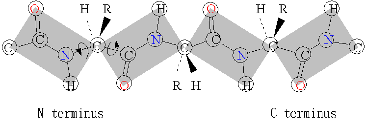
思路是比较简单的，就是找到一个蛋白质主链中的C,C\(_{\alpha}\),N,O这几种原子，然后计算对应共价键的二面角即可。计算相关内容可以参考我之前写过的这两篇文章：AlphaFold2中的残基刚体表示
和使用numpy计算分子内坐标。这里我们就简单的做一个Python的脚本，可以用来读取pdb文件，生成对应的拉氏图，用来判断对应的蛋白质构象是否合理，也可以用来比较两个同类蛋白之间的构型差异。

脚本与使用方法

先把下面这个Python脚本文件保存到本地为rplot.py：

# rplot.py
""" 
README
    Run this script with command:
    ```bash
    $ python3 rplot.py --input ../tutorials/pdb/case5.pdb --levels 8 --sigma 0.2 --grids 30
    ```
Requirements
    hadder, numpy, matplotlib
"""
try:
    from hadder.parsers import read_pdb
except ImportError:
    import os
    os.system('python3 -m pip install hadder --upgrade')
    from hadder.parsers import read_pdb
import matplotlib.pyplot as plt
import numpy as np

import argparse
parser = argparse.ArgumentParser()

parser.add_argument("--input", help="Set the input pdb filename. Absolute file path is recommended.")
parser.add_argument("--levels", help="Contour levels.", default='8')
parser.add_argument("--sigma", help="KDE band width.", default='0.2')
parser.add_argument("--grids", help="Number of grids.", default='30')

args = parser.parse_args()
pdb_name = args.input
num_levels = int(args.levels)
sigma = float(args.sigma)
num_grids = int(args.grids)

def plot(fig, X, Y, Z, num_levels=8):
    plt.xlabel(r'$\psi$')
    plt.ylabel(r'$\phi$')
    levels = np.linspace(np.min(Z), np.max(Z), num_levels)
    fc = plt.contourf(X, Y, Z, cmap='Greens', levels=levels)
    plt.colorbar(fc)
    return fig

def torsion(crds, index1, index2, index3, index4):
    crd1 = crds[index1]
    crd2 = crds[index2]
    crd3 = crds[index3]
    crd4 = crds[index4]
    vector1 = crd1 - crd2
    vector2 = crd4 - crd3
    axis_vector = crd3 - crd2
    vec_a = np.cross(vector1, axis_vector)
    vec_b = np.cross(vector2, axis_vector)
    cross_ab = np.cross(vec_a, vec_b)
    axis_vector /= np.linalg.norm(axis_vector, axis=-1, keepdims=True)
    sin_phi = np.sum(axis_vector * cross_ab, axis=-1)
    cos_phi = np.sum(vec_a * vec_b, axis=-1)
    phi = np.arctan(sin_phi / cos_phi)
    return phi

def psi_phi_from_pdb(pdb_name):
    pdb_obj = read_pdb(pdb_name)
    atom_names = pdb_obj.flatten_atoms
    crds = pdb_obj.flatten_crds
    c_index = np.where(atom_names=='C')[0]
    n_index = np.where(atom_names=='N')[0]
    ca_index = np.where(atom_names=='CA')[0]
    psi = torsion(crds, n_index[:-1], ca_index[:-1], c_index[:-1], n_index[1:])
    phi = torsion(crds, c_index[:-1], n_index[1:], ca_index[1:], c_index[1:])
    return psi, phi

def gaussian2(x1, x2, sigma1=1.0, sigma2=1.0, A=0.5):
    return np.sum(A*np.exp(-0.5*(x1**2/sigma1**2+x2**2/sigma2**2))/np.pi/sigma1/sigma2, axis=-1)

def potential_energy(position, psi, phi, sigma1, sigma2):
    # (A, )
    psi_, phi_ = position[:, 0], position[:, 1]
    # (A, R)
    delta_psi = psi_[:, None] - psi[None]
    delta_phi = phi_[:, None] - phi[None]
    # (A, )
    Z = -np.log(gaussian2(delta_psi, delta_phi, sigma1=sigma1, sigma2=sigma2, A=2.0)+1)
    return Z

psi_grids = np.linspace(-np.pi, np.pi, num_grids)
phi_grids = np.linspace(-np.pi, np.pi, num_grids)
grids = np.array(np.meshgrid(psi_grids, phi_grids)).T.reshape((-1, 2))
psi, phi = psi_phi_from_pdb(pdb_name)
Z = potential_energy(grids, psi, phi, sigma, sigma).reshape((psi_grids.shape[0], phi_grids.shape[0])).T
X,Y = np.meshgrid(psi_grids, phi_grids)

fig = plt.figure()
plt.title('Ramachandran plot for {}'.format(pdb_name.split('/')[-1]))
plot(fig, X, Y, Z, num_levels=num_levels)
plt.plot(psi, phi, '.', color='black')
plt.show()

然后加载一个本地pdb文件：

$ python rplot.py case2.pdb

生成图像效果如下：

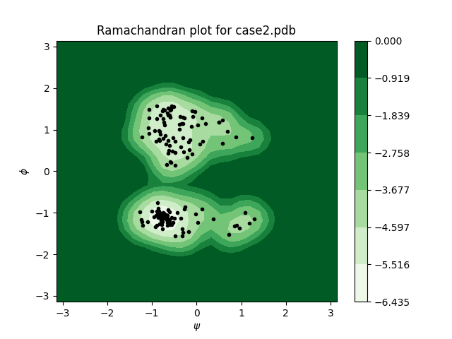
关于这个脚本还有一些常量可以配置：

$ python3 rplot.py --help
usage: rplot.py [-h] [--input INPUT] [--levels LEVELS] [--sigma SIGMA]
                [--grids GRIDS]

optional arguments:
  -h, --help       show this help message and exit
  --input INPUT    Set the input pdb filename. Absolute file path is
                   recommended.
  --levels LEVELS  Contour levels.
  --sigma SIGMA    KDE band width.
  --grids GRIDS    Number of grids.

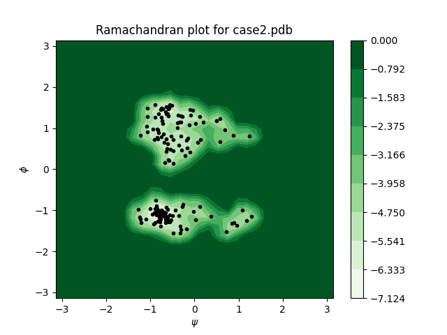
例如说，我们可以把KDE中高斯波包的sigma值配置的更小一点（默认值为0.2），这样图像显示的会更集中，还可以把levels调多一点（默认值为8），这样显示的等高线会更密一些：

$ python3 rplot.py --input ../tutorials/pdb/case2.pdb --sigma 0.1 --levels 10

效果如下：

总结概要

这里我提供了一个用于画拉氏图的Python脚本源代码，供大家免费使用。虽然现在也有很多免费的平台和工具可以用，但很多都是黑箱，有需要的开发者可以直接在这个脚本基础上二次开发，定制自己的拉氏图绘制方法。

版权声明

本文首发链接为：https://www.cnblogs.com/dechinphy/p/rplot.html

作者ID：DechinPhy

更多原著文章：https://www.cnblogs.com/dechinphy/

请博主喝咖啡：https://www.cnblogs.com/dechinphy/gallery/image/379634.html

参考链接

1. https://blog.csdn.net/MCANDML/article/details/80672174