ETJava Beta | Java
 注册
登录
注册
登录
注册
登录
注册
登录
上文有一些文字打错了,已经进行了修正。
本文主要介绍训练模型和使用模型预测数据,本文使用了一些numpy与tensor的转换,忘记的可以第二课的基础一起看。
首先使用datasets做一个数据X和y,然后结合之前的内容,求出y_predicted。
# pip install matplotlib
# pip install scikit-learn
import torch
import numpy as np
import torch.nn as nn
from sklearn import datasets
import matplotlib.pyplot as plt
# 0)准备数据
# 生成100行1列的数据X_numpy和Y_numpy
# noise=20: 值越大,数据越具有随机性。
# random_state=1: 设置随机种子,以确保每次生成的X_numpy和Y_numpy相同
X_numpy, Y_numpy = datasets.make_regression( n_samples=100, n_features=1, noise=20, random_state=1)

X = torch.from_numpy(X_numpy.astype(np.float32))
y = torch.from_numpy(Y_numpy.astype(np.float32))
y = y.view(y.shape[0], 1) #  100 行 1 列 y.shape是100行1列,所以y.shape[0]=100,y.shape[1]=1
n_samples, n_features = X.shape
# 1)模型
input_size = n_features
output_size = 1
model = nn.Linear(input_size, output_size)
# 2)损失函数和优化器
learning_rate = 0.01
criterion = nn.MSELoss()
optimizer = torch.optim.SGD(model.parameters(), lr=learning_rate)
n_iter = 100
#下面循环的调用了model里的前向传播和反复的使用损失函数进行反向传播来更新w和b,就是训练模型
for epoch in range(n_iter):
    # forward pass and loss
    y_predicted = model(X)
    loss = criterion(y_predicted, y)
    # backward pass
    loss.backward()
    # update
    optimizer.step()
    optimizer.zero_grad()
    if (epoch+1) % 10 == 0:
        print(f'epoch:{epoch+1},loss ={loss.item():.4f}')
# plot
# model(X).detach()是从model里分离出一个张量,这个张量跟model没有关系了,简单理解为生成了新张量对象,内存地址和model不一样了。
div_tensor = model(X).detach()
predicted = div_tensor.numpy() # 返回numpy.ndarray类型的张量,相当于转了类型
# plt.plot是在坐标系上绘制图像
# 参数1是x坐标轴的值,参数2是y坐标轴的值,参数3=是fmt (格式字符串)
# 参数3介绍:ro是红色圆点r=red o=circle  bo是蓝色圆点 b是蓝色 g是绿色
plt.plot(X_numpy,Y_numpy,'ro')
plt.plot(X_numpy, predicted, 'bo')
plt.show()
这里我们已经提到了训练的模型的概念了。
我们在for循环的调用了model里的前向传播,然后再反复的使用损失函数进行反向传播来更新w和b,这操作就是训练模型。
训练结束后,我们就可以使用model,接受新矩阵,来预测y。
这里,我们是在循环结束后,又使用我们训练的模型,重新对x进行了一次预测。
运行如下图:
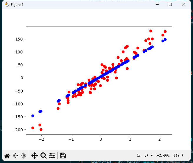
可以看到预测的y都在一条线上,这是因为预测值是基于w和b计算而得,所以,值总是在直线上。
注:所谓x和y的线性关系就是x和y的元素之间的很复杂的倍数关系。
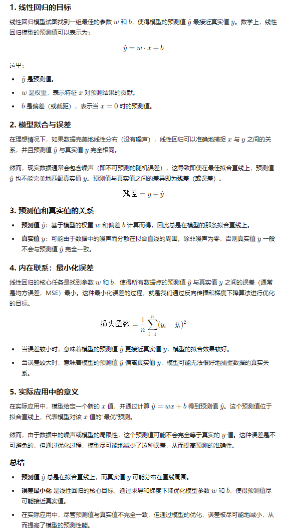
关于线性回归,可以参考下图,稍微了解一下就行。
下面是一个完整的训练模型,然后使用模型预测的例子。
首先使用datasets.load_breast_cancer()获取数据。数据X可以理解为一个患者的指标数据,Y可以理解为这个患者是否是癌症患者(数据都是0和1)。
然后通过训练模型,我们给一组患者的X指标数据,就可以预测患者是否是癌症患者了。
# pip install matplotlib
# pip install scikit-learn
import torch
import numpy as np
import torch.nn as nn
from sklearn import datasets
import matplotlib.pyplot as plt
from sklearn.preprocessing import StandardScaler
from sklearn.model_selection import train_test_split
# 0)prepare data
bc = datasets.load_breast_cancer() #加载乳腺癌数据集
print(bc.keys()) #data(特征数据)、target(标签)、feature_names(特征名)
X, y = bc.data, bc.target #取特征数据作为输入数据x(通常是一个二维数组或 DataFrame),取标签作为目标数据y(通常是一维数组或 Series)
print("x 569*30",X.shape,"y 569*1",y.shape)
n_samples, n_features = X.shape # n_samples=569 n_features=30
#train_test_split用于随机地将数据集拆分成训练集和测试
# X_train: 拆分后的训练集的特征部分,包含用于训练模型的大部分数据。
# X_test: 拆分后的测试集的特征部分,包含用于评估模型的小部分数据。
# y_train: 对应 X_train 的目标值,用于训练模型。
# y_test: 对应 X_test 的目标值,用于评估模型。
# test_size=0.2表示将 20% 的数据用于测试,剩下的 80% 用于训练
X_train, X_test, y_train, y_test = train_test_split(
X, y, test_size=0.2, random_state=1234)
print("X_train 455*30",X_train.shape,"X_test 114*1",X_test.shape,"y_train 455*1",y_train.shape,"y_test 114*1",y_test.shape)
print("类型1:X_train", type(X_train),"X_test", type(X_test),"y_train", type(y_train),"y_test", type(y_test))
# scale
# StandardScaler 用于对数据进行标准化(即缩放),缩放的方法是使用[标准化公式],
# 大概计算逻辑就是每个x调整为 (x-x集合的平均值)/根号((x-x集合的平均值)² )
# 经过标准化后,每个特征(特征=列)的均值会变为 0,标准差(平方差)变为 1。
sc = StandardScaler()
# fit_transform函数里会计算均值和标准差,然后下面的transform会使用fit_transform里的均值和方差
X_train = sc.fit_transform(X_train) #使用计算的均值和方差来标准化X_train
X_test = sc.transform(X_test) #使用fit_transform计算的均值和方差来标准化X_test
#x,y相关数据转tensor数组
X_train = torch.from_numpy(X_train.astype(np.float32))
X_test = torch.from_numpy(X_test.astype(np.float32))
y_train = torch.from_numpy(y_train.astype(np.float32))
y_test = torch.from_numpy(y_test.astype(np.float32))
print("类型2:X_train", type(X_train),"X_test", type(X_test),"y_train", type(y_train),"y_test", type(y_test))
print("X_train 455*30",X_train.shape,"X_test 114*1",X_test.shape,"y_train 455*1",y_train.shape,"y_test 114*1",y_test.shape)
# 转成tensor的y格式不对,进行view调整,原始size为torch.Size([114]) 调整后为:torch.Size([114, 1])
y_train = y_train.view(y_train.shape[0],1)
y_test = y_test.view(y_test.shape[0], 1)
# 1)model
# f=wx + b,sigmoid at the end
class LogisticRegression(nn.Module):
def __init__(self, n_input_features):
super(LogisticRegression, self).__init__()
self.linear = nn.Linear(n_input_features, 1) # 参数1:30(x的列)参数2:1(预测y的列)
def forward(self, x):
y_predicted = torch.sigmoid(self.linear(x)) #self.linear(x)执行的前向传播,sigmoid它将返回值转换为 [0, 1] 之间的概率值(概率值就是百分比,例如返回0.7,就是70%的意思)
return y_predicted
model = LogisticRegression(n_features)
# 2)loss and optimizer
learning_rate = 0.01
criterion = nn.BCELoss()
optimizer = torch.optim.SGD(model.parameters(), lr=learning_rate)
# 3)training loop
num_epochs = 100
for epoch in range(num_epochs):
# forward pass and loss
y_predicted = model(X_train)
loss = criterion(y_predicted,y_train)
# backward pass
loss.backward()
# updates
optimizer.step()
# zero gradients
optimizer.zero_grad()
if(epoch+1)% 10 == 0:print(f'epoch:{epoch+1},loss ={loss.item():.4f}')
# 模型的使用,这里是以前没有的
with torch.no_grad():
y_predicted = model(X_test) #把X_test传到模型里,得到X_test的预期y
y_predicted_cls=y_predicted.round() #四舍五入 y_predicted = torch.tensor([0.3, 0.7, 0.5, 0.2, 0.9]) y_predicted.round()的结果为: tensor([0., 1., 0., 0., 1.])
#eq(y_test): 这个方法比较 y_predicted_cls 和 y_test 之间的每个元素,如果两个值相等则返回 True,否则返回 False。返回的结果是一个布尔张量。
eq = y_predicted_cls.eq(y_test)
print("equal",eq)
eqsum = eq.sum()
print("eqsum",eqsum)
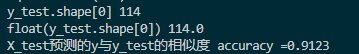
print("y_test.shape[0]", y_test.shape[0]) # y_test.shape[0]是 返回y_test的行,他原来是114行1列的矩阵,所以返回114
float_y_test= float(y_test.shape[0]) #转为float为下面除法准备
print("float(y_test.shape[0])", float_y_test)
acc=eqsum/float_y_test
print(f'X_test预测的y与y_test的相似度 accuracy ={acc:.4f}')
这样,我们不仅训练了模型,还使用模型预测了一组没有训练过的数据,并成功的预测出了,Y的值(患者是否是癌症),然后拿我们的预测数据,跟真实数据比较一下,正确率是91.23%
传送门:
零基础学习人工智能—Python—Pytorch学习(一)
零基础学习人工智能—Python—Pytorch学习(二)
零基础学习人工智能—Python—Pytorch学习(三)
零基础学习人工智能—Python—Pytorch学习(四)
零基础学习人工智能—Python—Pytorch学习(五)
注:此文章为原创,任何形式的转载都请联系作者获得授权并注明出处!

若您觉得这篇文章还不错,请点击下方的【推荐】,非常感谢!
 官方公众号
官方公众号